A Step-by-Step Case Study on Brain MRI Segmentation from Kaggle

12 min readSep 27, 2020

Figure 1: https://bitrefine.group/images/1920x870/mri_brain_1920x870.jpg

Business Problem
Deep Learning Architecture
Data Source
Existing Approaches
Improvements
Exploratory Data Analysis
Final Approach
Model Explanation
Code Snippets
Final Models Comparison
Future Work
References
Conclusion

Business Problem

Description

The case study is in reference to a segmentation based problem statement on the MRI scans of the human brain. The dataset primarily consists of images and their respective masks obtained from The Cancer Imaging Archive (TCIA) which corresponds to 110 patients included in The Cancer Genome Atlas (TCGA) lower-grade glioma collection.

Summary

The main purpose of the case study is to generate masks for the presence of cancerous tumors on the MRI scans of the human brain with the help of the given images and their respective masks. For this, we shall be using the LGG (Low Grade Glioma) Segmentation Dataset obtained from The Cancer Imaging Archive (TCIA)

Objectives

Our objective is to use the images and their corresponding masks in order to build an algorithm that correctly predicts the segmentation of cancerous tumors on the test images.
The evaluation metric we shall be using in this regard are DICE Coefficient as the loss function and IoU (Intersection over Union) as the accuracy-metric

Evaluation Metric

Dice Coefficient: Dice coefficient (DSC)is a measure of overlap between two sets. If two sets perfectly overlap, then the value of DSC is 1. Otherwise, DSC starts to decrease towards the minimum value of 0. In boundary detection tasks, the actual boundary pixels and the predicted boundary pixels can be defined as two sets. The numerator considers the overlap between the two sets at local scale while the denominator considers the total number of boundary pixels at global scale. If |X| and |Y| are the cardinalities of the two sets (i.e. the number of elements in each set), then:

IoU (Intersection over Union): Intersection over Union is an evaluation metric used to measure the accuracy of an object detector on a particular dataset. It is basically a ratio where in the numerator, we compute the area_of_overlap between the predicted bounding box and the actual bounding box. The denominator on the other hand, computes the area_of_union i.e. the area encompassed by both the predicted and actual bounding box. Since, the predicted bounding boxes that heavily overlap with the ground truth have higher scores than those with less overlap, so this makes IoU an excellent metric for evaluating custom object detectors.

Figure 3: https://i.imgur.com/SK5c0ng.png

Deep Learning Architecture

As a part of this case study, we shall be building a 2-step deep-learning pipeline in order to perform the segmentation task. It involves a binary classifier followed by a segmentation model where initially we shall be filtering the images for which mask is present (diagnosis=1) and then train all those filtered images using a segmentation model as represented below:

This will enable us to test the results faster as we are filtering our positive images (diagnosis=1) from the original data before sending it to the segmentation model.

Data Source

We are considering the LGG Segmentation Dataset as a part of this case-study with all the 7858 files including both images and masks as being provided by Kaggle to train our models. On closer analysis, we observe as follows:

All images are provided in .tif format with 3 channels per image.
For 101 cases, 3 sequences are available, i.e. pre-contrast, FLAIR, post-contrast (in this order of channels). For 9 cases, post-contrast sequence is missing and for 6 cases, pre-contrast sequence is missing. Missing sequences are replaced with FLAIR sequence to make all images 3-channel.
Masks are binary, 1-channel images.
The dataset is organized into 110 folders named after case ID that contains information about source institution. Each folder contains MR images with the following naming convention: TCGA_<institution-code>_<patient-id>_<slice-number>.tif Corresponding masks have a _mask suffix.

Existing Approaches

As per the available existing approaches, we could observe that a dataframe is being created initially consisting of the image_path and mask_path.
Once the dataframe is split into train & test, data-augmentation is being applied on the train-set using ImageDataGenerator from the tensorflow.keras library
Following this, the data is directly fed into a segmentation model which outputs the masks for all the corresponding input images.

Improvements

In addition to the image_path and mask_path columns, we shall be having another column as diagnosis which will be either 1 or 0 depending whether a mask is present (1) or absent (0) for a particular image
Instead of using ImageDataGenerator, we shall be building our very own data-pipeline using tf.data.Dataset for image-preprocessing and data-augmentation as shown below:

Our deep-learning architecture will basically consists of two models: a binary-classifier to predict the images having non-empty masks followed by a segmentation model which will be trained only on images for which mask is present (diagnosis=1)

Exploratory Data Analysis

Image-Mask Ratio

The primary task for us is to first analyze if for every given image-file, there exists a corresponding mask-file. In order to do so, we execute the following code snippet:

Since we know that in the given dataset there are a total of 7858 TIF files present and from the above code-snippet we observe that there are 3929 TIF files present for each of images and masks, hence we can conclude that for each MRI of a patient, there exists a corresponding mask for that image

Positive-Negative Diagnosis

As a part of this case study, we shall be first performing classification based on the image being positive (diagnosis=1) or negative (diagnosis=0). In order to do so, we are adding another column diagnosis in the dataset as follows:

The diagnosis is computed by analyzing the presence of empty masks using the function as shown below:

From the pie-plot represented below, we can observe that 35% of all the masks have a positive diagnosis and the remaining 65% have a negative diagnosis:

Figure 9: Pie Chart for Diagnosis Distribution

Positive Masks: The figure below represents a set of MRI images for which mask is present. i.e. diagnosis=1

Negative Masks: The figure below represents a set of MRI images for which mask is absent. i.e. diagnosis=0

Here we have observed that if the diagnosis is positive then we have a distinct segmentation present for the respective masks. But if the diagnosis is negative, then there is no segmentation present for the given masks

Binary Classification Analysis

In order to pose our problem statement as a binary classification task, we need to first analyze if all the values in the mask files are zero. For this we randomly pick some mask files with diagnosis=0 and then compute the max-min values of the files using the code-snippet as shown below:

Figure 12: Max-Min Pixel Values of Masks

Here we can conclude that since the the pixel values of all the masks with negative values have been observed to be zero (0), hence we can pose this problem initially as binary classification based to segregate the positive and negative images and later perform segmentation on the positive ones

Final Approach

Step I: Binary Classification

Following a 80:20 ratio, we shall be first splitting the dataset into train and test which will basically lead to the training set consist of 3143 datapoints while the test dataset shall comprise of 786 datapoints.
For the binary-classification task, we shall be considering only the image_path and diagnosis columns of the dataset.
As a part of the data-preprocessing step, each image is normalized and then resized to pixel values of 256 x 256
Data augmentation is another step which we shall be following in order to significantly increase the diversity of data available for training models.
In addition to the accuracy metric, we shall be monitoring three other metrics as well viz. recall, precision and f1_score
Out of all the actual positive points, the recall metric will determine what percentage of them are predicted to be positive by the model. Out of all the points the model predicted to be positive, the precision metric will determine what percentage of them are actually positive. Since we want both the recall and the precision to be high, so we shall monitor the f1_score too which should also be high.
The classification model we shall be using in this regard is the Xception architecture. However, we won’t be using any pre-trained weights in this regard but rather train the model with our own dataset
On training the model, we observe the best scores with accuracy and val_accuracy to be 0.9252 and 0.9160 respectively. Hence, we can conclude that the model is not overfitting and consider this to be the best-model with recall and precision values to be 81% and 93% respetively. Furthermore, the f1_score is also observed to be 86%

Step II: Image Segmentation

Here, instead of training the entire dataset, we shall be considering only those datapoints with diagnosis=1. As such with a 80:20 split, we are left with 1098 datapoints for train and 275 datapoints for test
As for model-training, we are taking into account the image_path and mask_path columns of the dataset.
Like in the previous step for binary-classification, here also we shall be performing normalization and resizing on the images as well as to their respective masks as a part of data-preprocessing followed by augmentation
The performance mentric we shall be monitoring in this regard are dice-coefficient as the loss-function and intersection over union for model acuracy
The model architectures that we are going to experiment with as a part of the image segmentation task are UNet and UNet++. Here also, we are not using any pre-trained weights for both the architectures

Model Explanation

Xception

The Xception model is inspired from Google’s Inception model. The architecture follows a linear stack of depthwise separable convolution layers with residual connections (skip connections).

The depthwise separable convolution basically involves a combination of 3 x 3 spatial convolutions for each channel followed by 1 x 1 depthwise convolutions on concatenated channels. In order to get a better clarity of the depthwise separable convolution, we can consider the example as mentioned below:

Let us consider a 3 x 3 convolution layer on 16 input channels and 32 output channels.
In case of regular convolution, the total number of parameters = 16 * 32 * 3 * 3 = 4608
But for depthwise separable convolution, the number of parameters = (spatial_conv + depthwise_conv) = (16 * 3 * 3 + 16 * 32 * 1 * 1) = 656

The Xception architecture is represented below:

Figure 13: https://miro.medium.com/max/600/1*459jKxLPM9R-Y_z0y8SXug.png

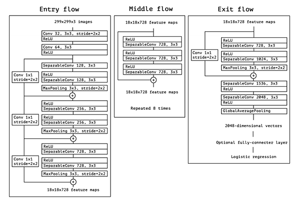
Entry Flow: It comprises of two conv_block followed by three xception_block as shown below:

Middle Flow: It comprises of eight middle_flow_block stacked one after the other as shown below:

Exit Flow: It comprises of an xception_block followed by two separable_conv_block, a GlobalAveragePooling layer and then the desired custom layers as per the output required:

UNet

The UNet model creates a pixel-wise mask of each object in the images. The goal is to identify the location and shapes of different objects in the image by classifying every pixel in the desired labels. One of the main advantage of using UNet is that it can be trained end-to-end with fewer training samples and still yield more precise segmentations which is very critical for medical images

The UNet architecture is represented below:

Figure 17: https://miro.medium.com/max/2824/1*f7YOaE4TWubwaFF7Z1fzNw.png

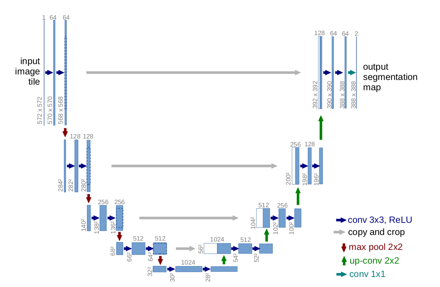
Downsampling: Each downsampling step comprises of two 3 x 3 convolutions (blue arrow) followed by a 2 x 2 max-poooling (red arrow) where the number of channels are doubled as shown below:

Upsampling: Each upsampling step comprises of a 2 x 2 up-convolution (green arrow) concatenated with the feature maps of the corresponding layer from downsampling (gray arrow) to provide localization due to the loss of border pixels in every convolution. It is then followed by two 3 x 3 convolutions (blue arrow) where the number of channels are halved as shown below:

UNet++

The UNet++ model follows the basic structure and principle of the UNet model however with the exception that it tries to further improve the segmentation accuracy by including dense_block and convolution layers between the encoder and decoder.

The UNet++ architecture is represented below:

Figure 20: https://miro.medium.com/max/658/1*ExIkm6cImpPgpetFW1kwyQ.png

Redesigned Skip Pathways: The redesigned skip pathways (shown in green) have been added to bridge the semantic gap between the encoder and decoder subpaths. Following code snippet represents the pathway x2_0 → x1_1 → x0_2 as shown below:

Dense Skip Connetions: The dense skip connections (shown in blue) ensures that all prior feature maps are accumulated and arrive at the current node because of the dense convolution block along each skip pathway. Following code snippet represents the pathway x1_0 → x1_1 → x1_2 → x1_3 as shown below:

Deep Supervision: The deep supervision (shown in red) is added to adjust the model complexity between speed and performance. For accuracy, the output from all segmentation branch is averaged whereas for speed, the final segementation map is selected from one of the segmentation branches.

Code Snippets

The plot_hist(df, text) function is being used for generating the count-plot of each of the target labels present in the dataset

The parse_data(image_path, label) function is being used for performing image-preprocessing tasks like normalization and resizing on each of the image files

The augment_data(image, label) function is being used for applying data-augmentation techniques like flip and brightness on each of the image files

Final Models Comparison

While training the two segmentation models, we did not observe very high difference in the validation iou-scores with UNet generating a val_iou of 0.807 and UNet++ generating a val_iou of 0.808

On closer analysis, we compared the predicted masks as generated by UNet and UNet++ with the ground-truth mask on the test dataset and observed as follows:

Future Work

In addition to the Xception model which we have used as a binary classifier, we can also also experiment with other architecture like SqueezeNet to try and improve the accuracy scores.
As a part of the image-segmentation task, we observed that the number of training samples is quite low. Performing some more data-augmentation techniques in addition to what we have used may lead to improve the iou_scores further.
For both the models, we can further try to improve the scores by reducing the learning_rate of the optimizers while training the models as a callback when it starts to plateau

References

Conclusion

All files related to the codes for the end-to-end implementation of the whole case study is available on Github which can be accessed by clicking on Github

References

- https://medium.com/ai-salon/understanding-dice-loss-for-crisp-boundary-detection
- https://www.pyimagesearch.com/2016/11/07/intersection-over-union-iou-for-object-detection/
- https://stephan-osterburg.gitbook.io/coding/coding/ml-dl/tensorfow/ch3-xception/xception-architectural-design
- https://jinglescode.github.io/2019/11/07/biomedical-image-segmentation-u-net/